
Learning Thermodynamics through Jupyter Notebook (Python)?
As part of the course MCG 2530 – Thermodynamics 1 (Fall 2025 semester), Part B (optional) of the assignments was designed to progressively introduce students to the use of Jupyter Notebook (Python) as a tool for analysis and modeling in thermodynamics. Unlike traditional paper-and-pencil exercises, these activities emphasize:
- the numerical solution of thermodynamic equations,
- the visualization of results (diagrams, curves, model comparisons),
- and, most importantly, a direct connection to real engineering problems, inspired by industrial practice and research.
Students work in an interactive environment combining code, equations, plots, and written commentary, reflecting modern methods commonly used in mechanical, energy, and environmental engineering.
🔹 Assignment D1.B – Introduction to Jupyter Notebook and Computational Thermodynamics
Students are introduced to Jupyter Notebook and core Python libraries (NumPy, Matplotlib, Cantera). Through concrete examples, they learn to:
- explore the thermodynamic properties of real substances,
- plot T–v and P–v diagrams,
- analyze supercritical fluids and their engineering constraints.
Objective: establish the foundations of numerical computation applied to thermodynamics.
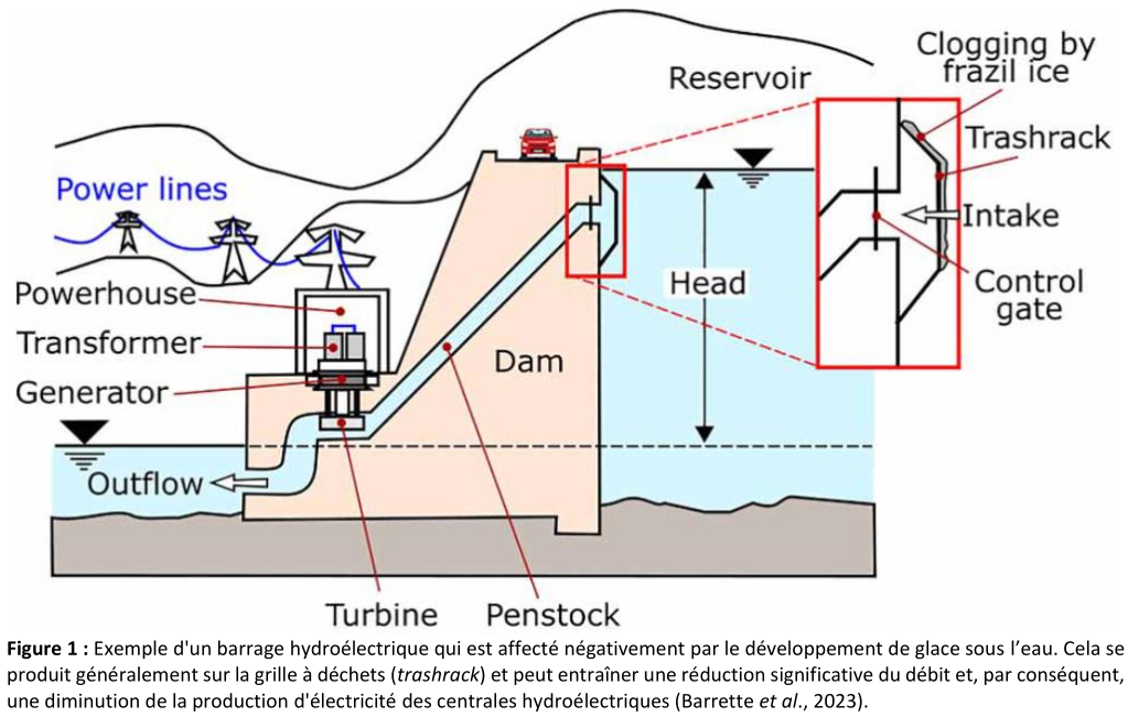
🔹 Assignment D2.B – Frazil Ice Mitigation in Hydroelectric Power Plants
This assignment is based on a critical real-world problem in Canada: the formation of frazil ice at water intakes. Students use Python to compare two industrial mitigation strategies:
- water heating,
- compressed-air bubbling systems.
They estimate energy requirements, compare costs, and discuss the underlying physical assumptions.
Objective: connect thermodynamics to concrete energy and environmental challenges.
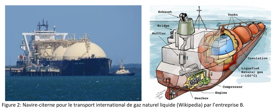
🔹 Assignment D3.B – Ideal Gases, Real Gases, and Natural Gas Compression
Inspired by the industrial transport of natural gas, this assignment requires students to:
- compare the ideal gas model with a real gas model (using Cantera),
- evaluate compression work up to 200 bar,
- estimate the actual energy cost of compressed gas transport.
Objective: understand the limitations of idealized models in an industrial context.
🔹 Assignment D4.B – Laser-Induced Incandescence (LII): Closed System
This assignment introduces a problem drawn from combustion research and laser diagnostics. Students develop a numerical model to predict the time-dependent temperature evolution of a soot particle exposed to a laser pulse by solving a transient energy balance.
Objective: apply the first law of thermodynamics to a microscopic transient system using numerical methods.
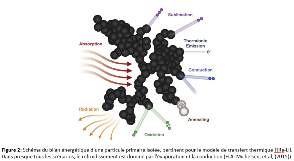
🔹 Assignment D5.B – Laser-Induced Incandescence (LII): Open System
Building on Assignment D4, this final assignment extends the model by introducing particle sublimation, transforming the problem into an open system with mass loss. Students simultaneously model:
- temperature evolution,
- mass loss,
- particle diameter variation.
Objective: concretely illustrate the difference between closed and open systems in an advanced research context.
The use of Jupyter Notebook throughout these assignments enables students to:
- develop scientific programming skills,
- work with realistic physical models,
- adopt practices closely aligned with those used in research and industry.
This approach promotes a deeper understanding of thermodynamics beyond equations alone, by demonstrating how fundamental concepts translate into practical analytical tools.
Acknowledgments
These activities would not have been possible without the engagement, motivation, and dedication of the students who actively participated in completing the assignments. I thank all students for their commitment. Special recognition is given to Shea Kennedy and Mateo de Grace for the exceptional quality of their work!